Exploring Polynomial Regression
Algorithm ·Polynomial Regression is the generalization of Linear Regression to polynomial function. In Linear Regression, we fit a straight line (i.e. \(y=f(x)=mx+c\)) to our dataset. Here, in Polynomial Regression, we fit a polynomial function of \(x\) to the data. The polynomial function of \(x\) is as follows:
\(y=f(x)=a_{0} + a_{1}x + a_{2}x^2 + \cdots + a_{n}x^n\)
Where, \(a_{n}\) is the coefficient of order n and \(x^n\) is the \(n^{th}\) power of input \(x\).
This post on Polynomial Regression heavily relies on the concept developed on Linear Regression Post.
Python (Jupyter) Notebook of Polynomial Regression is on this Github Repository. You can also run the Notebook on Google Collab
Why use Polynomial Regression?
According to Stone–Weierstrass theorem, every continuous function defined on a closed interval [a, b] can be uniformly approximated as closely as desired by a polynomial function. A polynomial function of order n (highest degree of \(x\)) < m (number of data points) can fit the data approximately (or exactly when \(n = m-1\)).
Linear Regression fits the \(1^{st}\) order polynomial (line) of the form \(y=a_{0} + a_{1}x\) to the data. Using Polynomial Regression of higher-order, we can fit a curve to our data rather than just straight line. Since fitting a straight line is not always appropriate to our dataset, we use polynomial regression in general.
What does a Polynomial Function look like?
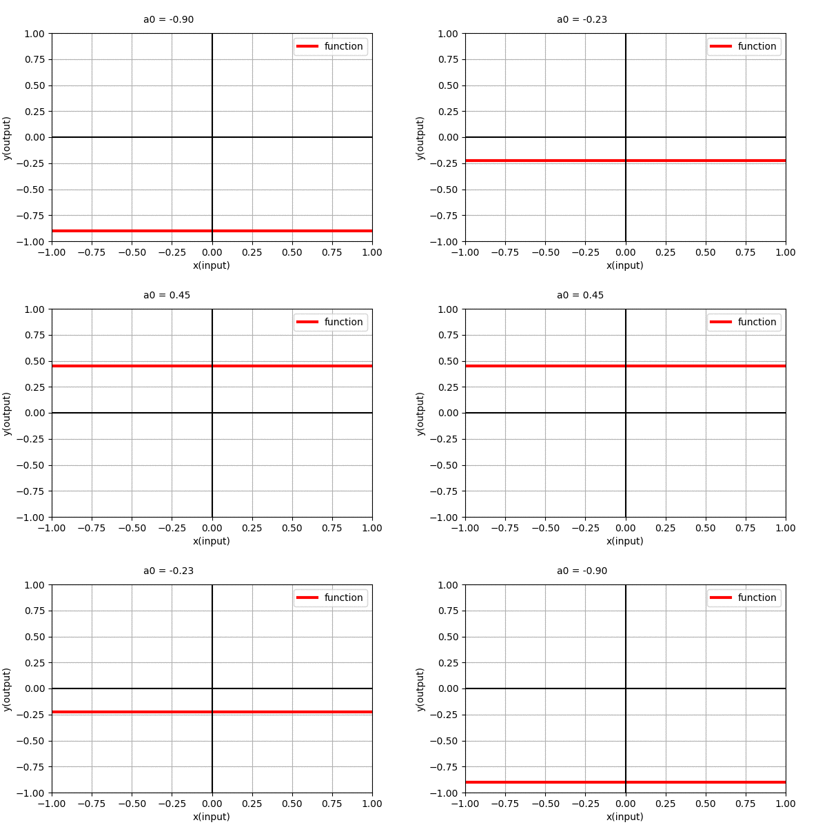
Polynomial of degree 0 ,i.e. \(y=a_{0}\) is a straight line parallel to x-axis. We can see that it is independent of \(x\). The dynamics of the parallel line with varying coefficient can be seen in the figure below.
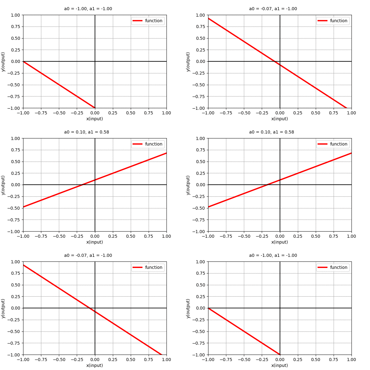
Polynomial of degree 1 i.e \(y=a_{0} + a_{1}x\) is a line with slope \(a_{1}\) and y-intercept \(a_{0}\). The dynamics of line with varying coefficients can be seen in the figure below.
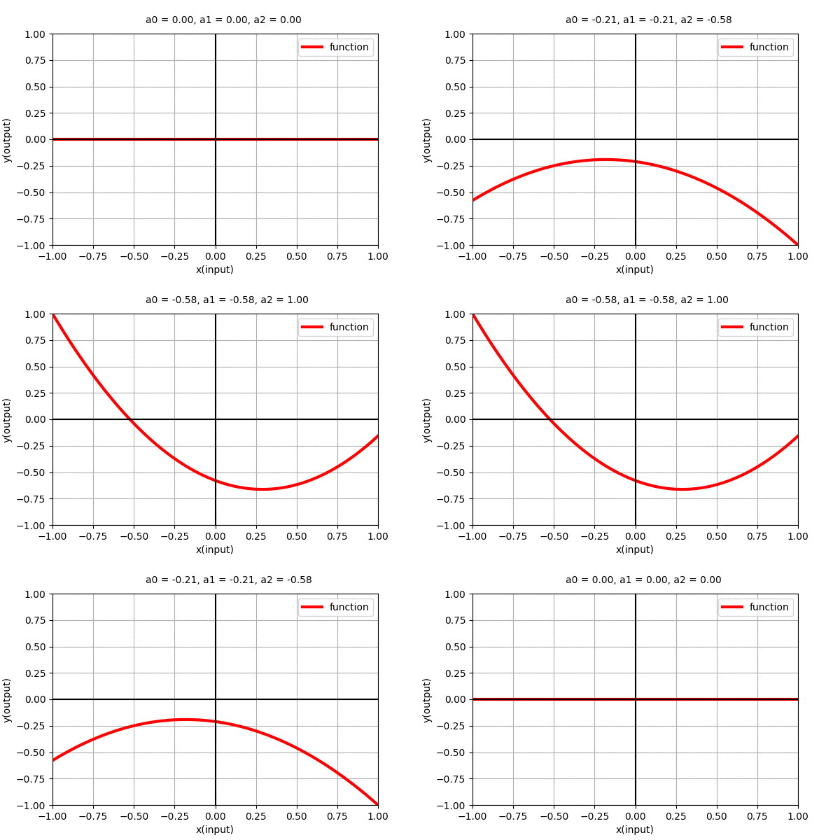
Polynomial of degree 2 i.e \(y=a_{0} + a_{1}x + + a_{2}x^{2}\) is a parabolic curve with one maxima/minima. Similarly, here also, we can see the dynamics of the curve with varying coefficients as shown in the figure below.
Similarly, Polynomial function of degree \(n\) i.e. \(y=f(x)=a_{0} + a_{1}x + a_{2}x^2 + \cdots + a_{n}x^n\) is a curve with \(n-1\) minima/maxima (wiggles). Let us see what type of functions do higher order polynomial functions represent.
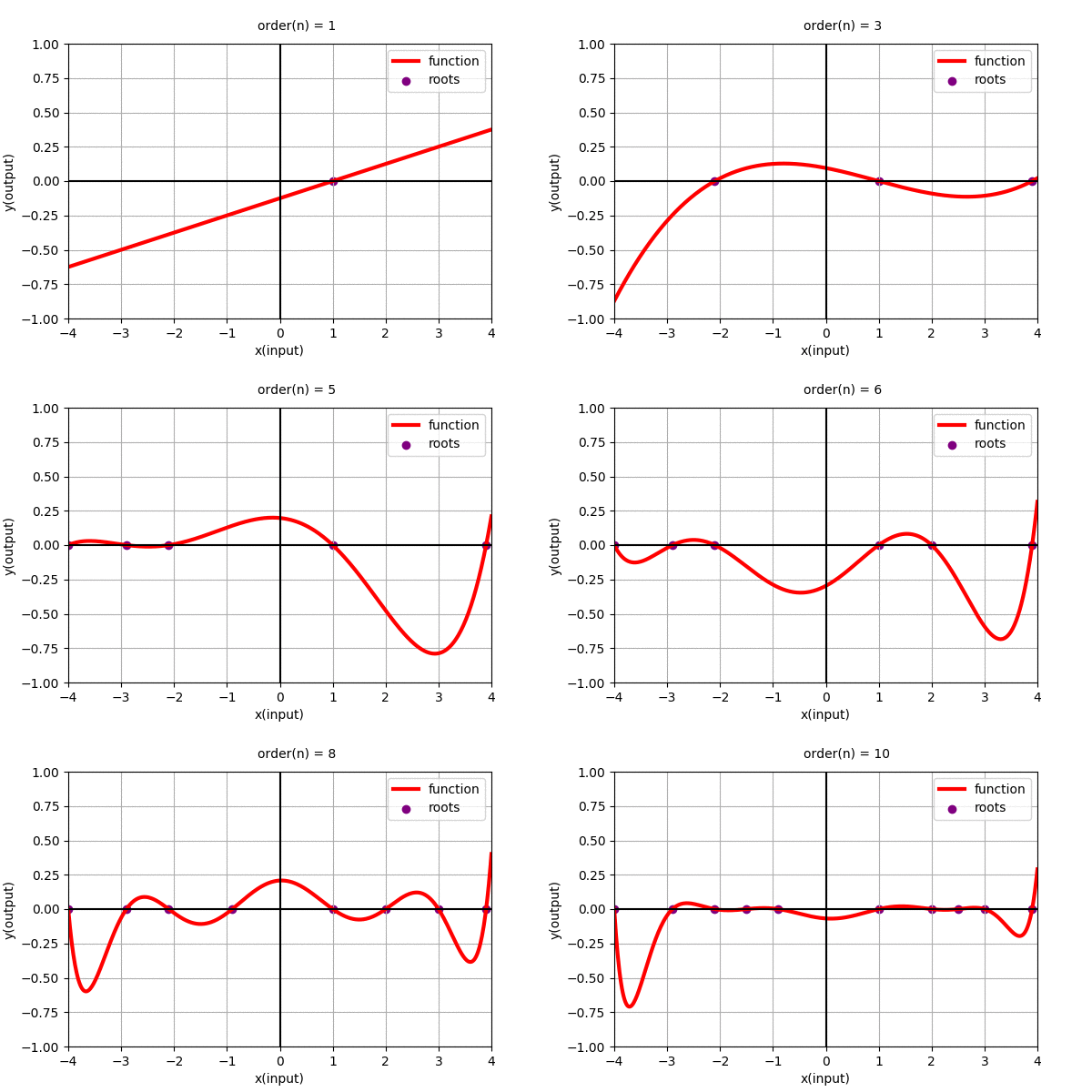
In the above figure we found the polynomial function using roots. Polynomial function can be alternatively represented as: \(y=f(x)=c(x-x_{0})(x-x_{1})(x-x_{2})(x-x_{3})\cdots(x-x_{n-1})\)
where, \(x_{i}\) for i = 0 to n-1, are the roots of the polynomial function and c is the constant scaler to the overall function. (Roots are the values of \(x\) where the value of the function, \(y=f(x)\) are zero.)
Now, Let’s get back to our problem of fitting the above curvy data points.
How do we find the coefficients of Polynomial Regression?
The method of finding the coefficients of Polynomial Regression is very similar to that of Linear Regression. The problem can be reformulated as multivariate linear regression with input vectors composed of various powers of input \(x\). A single input \(x_{0}\) can be represented as a vector(column matrix) \(\boldsymbol{x_{0}}\) consisting of various powers of \(x_{0}\) as below.
\[\boldsymbol{x_{0}}= \begin{bmatrix} 1 \\ x_{0} \\ x_{0}^{2}\\ x_{0}^{3}\\ \vdots \\ x_{0}^{n} \end{bmatrix}\]Using this form, we can compute the Polynomial function for given input \(x_{0}\), given a coefficient matrix A as follows.
\[\begin{align*} \boldsymbol{y_{0}} &= \boldsymbol{x_{0}}.\boldsymbol{A} \\ &= a_{0} + a_{1}x + a_{2}x^2 + \cdots + a_{n}x^n \end{align*}\]Where, the coeffecient matrix \(\boldsymbol{A}\) is as follows:
\[\boldsymbol{A}= \begin{bmatrix} a_{0} \\ a_{1} \\ a_{2}\\ \vdots \\ a_{n} \end{bmatrix}\]Since we are finding the polynomial function to fit all the data points, we use all the input points with their various powers as input. We can easily do Linear Regression with multiple variables using Matrices. So, let us write our polynomial function as Matrix Algebra as follows:
\[\boldsymbol{Y} = \boldsymbol{X}.\boldsymbol{A} \tag{1}\]where,
\[\boldsymbol{X}= \begin{bmatrix} \boldsymbol{x_{0}^{T}}\\ \boldsymbol{x_{1}^{T}}\\ \vdots\\ \boldsymbol{x_{n}^{T}} \end{bmatrix} = \begin{bmatrix} 1 &x_{0} &x_{0}^{2} &\cdots &x_{0}^{n} \\ 1 &x_{1} &x_{1}^{2} &\cdots &x_{1}^{n} \\ \vdots &\vdots &\vdots &\ddots &\vdots \\ 1 &x_{m-1} &x_{m-1}^{2} &\cdots &x_{m-1}^{n} \\ \end{bmatrix}\]Here, we are dealing with 1D input only. The input matrix consists of various powers of each input in each \(i^{th}\) rows. The \(j^{th}\) column consists of \(j^{th}\) power of input data. So, each row can be considered as single a input vector and each column as data points of a single feature. With these features, multivariate linear regression is performed.
\[\boldsymbol{A}= \begin{bmatrix} a_{0} \\ a_{1} \\ a_{2}\\ \vdots \\ a_{n} \end{bmatrix} \hspace{1mm} and \hspace{2mm} \boldsymbol{Y}= \begin{bmatrix} y_{0} \\ y_{1} \\ y_{2}\\ \vdots \\ y_{m-1} \end{bmatrix}\]For the coefficient matrix, each column represents coefficients for each output features and each row represent the coefficients for each input features. Since we have used a single output feature, we have only one column.
For the output matrix, each row is the output vector/constant of each input vector, the number of columns represents the number of output features. Since we have a single output feature, we have one column of the output matrix.
Here, \(\textbf{X} \in \mathbb{R}^{m\times (n+1)} ;\qquad \textbf{W} \in \mathbb{R}^{(n+1)\times 1} ; \qquad\textbf{Y} \in \mathbb{R}^{m\times 1}\)
The equation (1) can be solved for \(\boldsymbol{A}\) using a little bit of Matrix Algebra, as we did on Linear Regression.
\[\begin{align*} \textbf{Y} &= \textbf{X} . \textbf{A} \\ \textbf{X}^{+} . \textbf{Y} &= \textbf{X}^{+} . \textbf{X} . \textbf{A} \\ \textbf{X}^{+} . \textbf{Y} &= \textbf{I} . \textbf{A} \\ \textbf{A} &= \textbf{X}^{+} . \textbf{Y} \tag{2} \end{align*}\]Here, \(\textbf{X}^{+}\) is the Moore–Penrose pseudoinverse of matrix \(\textbf{X}\) and \(\textbf{I}\) is the identity matrix.
Now, we know how to do polynomial regression, let’s try fitting polynomial function to our dataset.
Second order Polynomial Regression
Let us consider a dataset (same as we used in Linear Regression). We previously fit a straight line to the data, as shown in the figure below.
As can be seen in the visualization, we expect the function to be little curvy to exactly approximate the function.
With the above-mentioned method, lets first define our matrices \(\boldsymbol{X}\), \(\boldsymbol{A}\) and \(\boldsymbol{Y}\).
Since we have 200 data points, 3 input features and 1 output features, we have our matrices as follows.
Here, \(\textbf{X} \in \mathbb{R}^{200\times 3} ;\qquad \textbf{A} \in \mathbb{R}^{3\times 1} ;\qquad \textbf{Y} \in \mathbb{R}^{200\times 1}\)
We can construct input matrix \(\boldsymbol{X}\) easily and we have output matrix \(\boldsymbol{Y}\), We can now calculate the Coefficient Matrix \(\boldsymbol{A}\) by using the equation (2). Doing so, we get:
\[\boldsymbol{A}= \begin{bmatrix} 0.7784 \\ 0.3381 \\ -0.4601 \end{bmatrix}\]The plot of the second order polynomial (learned) that best fits the data, represented by the coefficients, is shown in the figure below:
Well, this looks prettttyyyy good fit. The mean squared error of this fit is \(E=0.000807\) which is smaller than the linear regression case of \(E=0.002033\). (We have a great tool that can approximate any function. Is this all we need for regression/curve fitting?)
We have accomplished the goal to fit a curve to our dataset. The function learned is curvy, but we don’t consider polynomial regression as non-linear regression. This is because, it is the special case of multivariate linear regression, where the inputs are various powers of \(x\).
Higher order Polynomial Regression
We can fit higher order polynomial to our dataset. Since we have 200 data points, we can fit, at highest, 199 order polynomial to our dataset. Let’s see how the polynomial regression of various order fit our dataset. Let us see how different order Polynomial Regression on our dataset looks like.
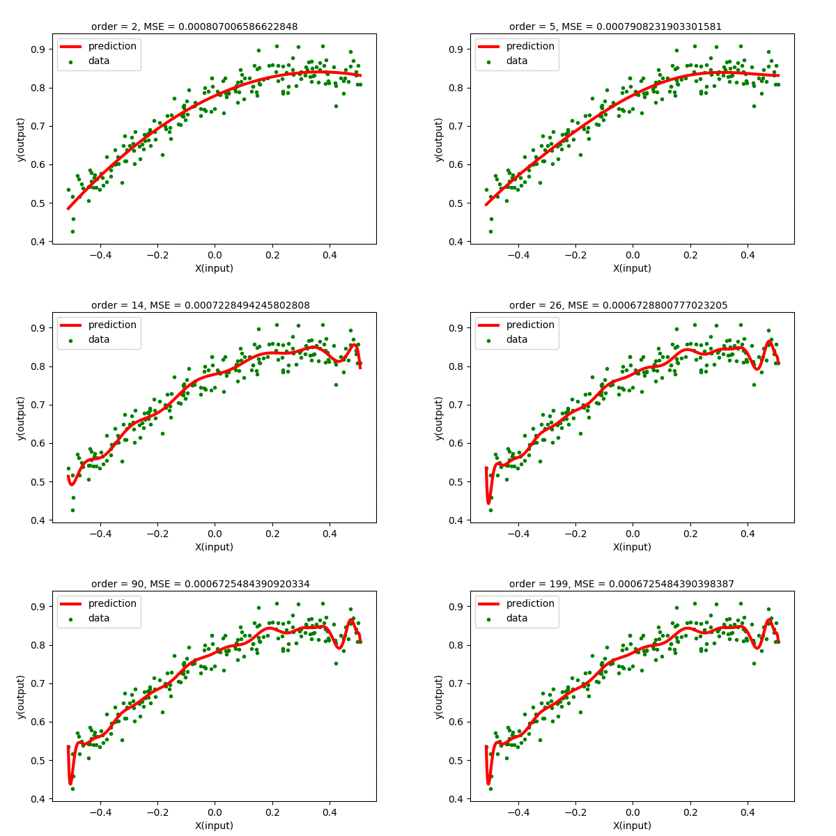
The error plot of various degree of polynomial can be observed as below.
We can see that the higher order polynomial function produces lower and lower error as order increases. The problem is that the curve gets more wiggly as the degree of polynomial increases. This is not what we want. We want the simplest curve to fit our data.
Humm… We were expecting to have zero error for 199 degree polynomial, but the curve looks the same for higher order polynomials. We know that, using Polynomial Interpolation we can fit every point to the polynomial function. This is just linear regression, so nothing fishy is going here. Maybe the problem is in the data. Let’s analyze the data, i.e different powers of \(x\). Following is a visualization of \(x^{n}\) for n in (0,1,2,…).
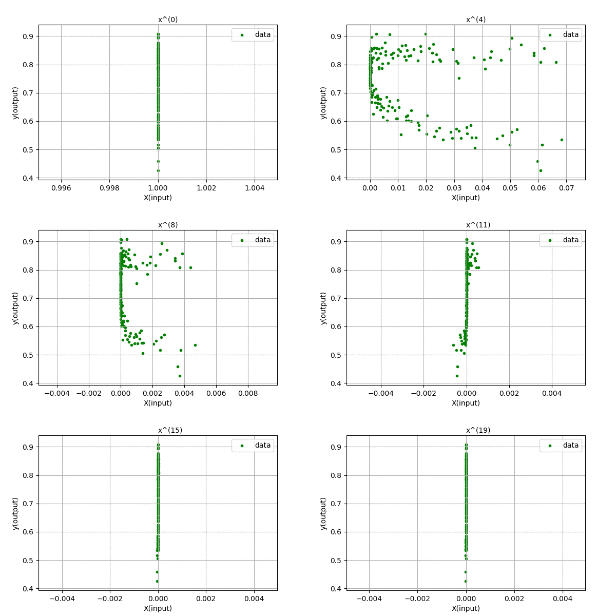
We can see that the input feature, \(x^{n}\) tends to zero as the degree of polynomial increases. This is because we centered out data in [-0.5,0.5] range. The magnitude of each value is less than 1, and higher the value of n, smaller the feature values. Thus, the data range is so small that even float64 data cant handle accurately storing and representing the data. There are also errors related to computing pseudo-inverses of the matrix. When the magnitude of data is greater than 1, its higher power grows towards infinity. Our method is not faulty, we only hit the limitation of our computation.
We got lost in something else here.. Our previous problem is not solved.
What is the problem?
We want to get the objective of having a minimum error fit. Having minimum error should obviously be better, isn’t it?. Maybe our objective function itself is our problem. We have got the least error, but still, we did not get the desired model of the data. Something is lacking in our problem formulation. The error is minimum (zero in theoretical case) for order of 199, but that is not the best representation of the data. It just fits every point by doing Polynomial Interpolation. We want the simplest best fit model of the data, not the least error one. This is what Occam’s razor suggests.
Why do we need the simplest model? Wouldn’t the overfit model do the job?
Generally, with the functional model of the data, we use it to predict previously unseen data in the future. This is what most machine learning algorithms are used for. Hence, we should incorporate the notion of usability for the future as well as the simplicity of the function learnt to determine the best possible solution.
This algorithm has solved the problem of non-linear curve fitting but has added more problem of model complexity, computational constraints, selecting the degree of polynomial \(n\) (hyperparameter).
How do we determine the best degree of polynomial?
The degree of polynomial determines the number of parameters and the complexity(capacity) of the function learnt. The linear regression case is simple because there is only one possible way to do it. But, in polynomial regression, there is an overhead of determining the degree of polynomial (hyperparameter). There is no straightforward way to determine the exact degree of polynomial required. This can only be done by general hyperparameter tweaking methods. This includes searching over the space of hyperparameters.
Let us tackle this problem by simplifying our dataset. Let’s use a case where we have 5 points roughly following a curve. The various degree of curves fitted to the dataset is shown in the figure below.
All these curves are trying to fit the data, but how do we choose the most appropriate one? It seems that the polynomial function of order 2 is the simplest and fits the data satisfactorily. The order 4 polynomial function perfectly fits all the training data, but it does not generalize well.
We can construct a solution to this problem by using another set of data, to test how the prediction accuracy results. This dataset is called test dataset. We will find the error of the model on this dataset and hence conclude that the model with least test error is the best one. This is because the model that does better prediction on an unseen dataset is what we are practically trying to achieve.
This choice of model complexity is another fundamental problem in machine learning, called Bias-Variance tradeoff. It says that we can fit a simple model but the test and train error will be high… and/or …we can fit a complex model to have low train error, but the test error will be high. We have to find the sweet spot between the simple model and complex model where the test error is lowest. This helps our model to generalize well. This problem can be taken as a generalization problem, that can be tweaked by changing model complexity. The test of generalization is done by using a test dataset.
Hence, we can find the best degree of a polynomial using this method. It is easy to find the optimal value of hyperparameter by searching over the range of possible values. The search is for the least test error case.
This concept is more intuitive when if we plot the train and test error curve. Let’s do that with our own dataset.
What is the best degree of polynomial to fit our dataset?
Let’s use the above mentioned method of using test dataset to determine the best degree of the polynomial. For this, we need test-dataset. Let us generate the test-dataset from same function as train-dataset.
We will do the same fits as we did previously in our dataset. This time we will keep a record of all the train set error and test set error to make a comparison.
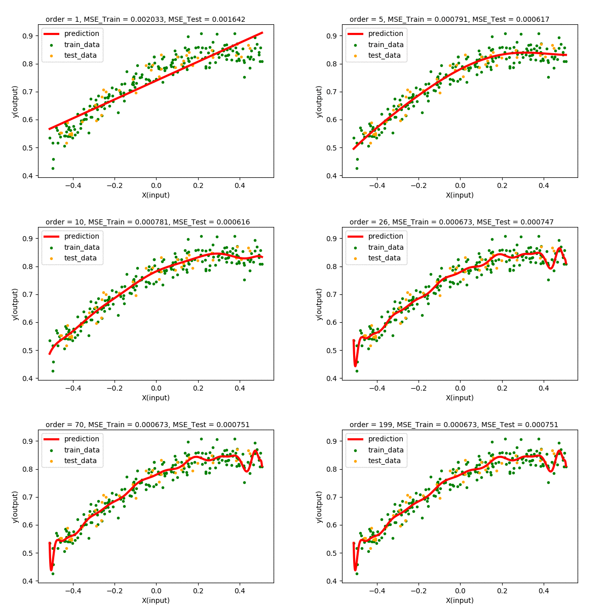
Let’s summarize our observations by plotting all the train and test error values of various degrees of polynomial regression.
We can see that up to some point (2 in our case), the train and test error decreases when increasing the degree of the polynomial. After that, we will have higher and higher test error, although the training error decreases continuously. Hence, we pick the point of lowest test error with the least complexity. In our case, we pick the polynomial function \(y=f(x)=0.778+ 0.338x-0.46x^{2}\) of order 2 as the best model of our dataset.
We can follow the same method on any dataset where we want to perform curve fitting. For now, let’s explore another method of doing Polynomial Regression: Gradient Descent.
Polynomial Regression using Gradient Descent
We previously used the matrix inversion technique to find the parameters matrix A. We can also find it by using the gradient descent search technique. This method will come handy when there are large number of parameters and computing inverse matrix is not feasible.
We have the equation,
\[\boldsymbol{\hat{Y}} = \boldsymbol{X}.\boldsymbol{A} \tag{3}\]In gradient descent, we find the error and then find the gradient of the parameters with respect to (w.r.t) the error function.
We can do the same for finding the whole parameter matrix using linear algebra and calculus.
The error function is still the same Mean Squared Error (modified). We know that the mean squared error is:
\[E(\boldsymbol{A}) = \frac{1}{2n}\sum_{i}{e_{i}^2}\]In our case, we have only one output feature and 200 data points, hence the output is columnar matrix. The error function can be written as:
\[\begin{align*} E(\boldsymbol{A}) &= \frac{1}{2n}\sum_{i=0}^{m-1} e_{i}^2 \\ &= \frac{1}{2n}\sum_{i=0}^{m-1} (\hat{y_{i}} - y_{i})^2 \tag{4} \\ \end{align*}\]Differentiating equation (4) w.r.t \(\hat{y_{i}}\) for i = 0 to m-1, we get:
\[\begin{align*} \frac{dE}{d\hat{y_{i}}} &= \frac{1}{n}(\hat{y_{i}} - y_{i}) \\ &= \frac{1}{n} \Delta y_{i} \end{align*}\]We can write this in columnar matrix form as:
\[\begin{align*} \begin{bmatrix} \frac{dE}{d\hat{y_{0}}} \\ \frac{dE}{d\hat{y_{1}}} \\ \vdots \\ \frac{dE}{d\hat{y_{m-1}}} \end{bmatrix} &= \frac{1}{n} \begin{bmatrix} \Delta y_{0} \\ \Delta y_{1} \\ \vdots \\ \Delta y_{m-1} \end{bmatrix}\\ or,\hspace{2mm} \frac{dE}{d\boldsymbol{\hat{Y}}} &= \frac{1}{n} \Delta \boldsymbol{Y} \tag{5} \end{align*}\]Here, we have computed the gradient of the Error Function w.r.t the output matrix \(\boldsymbol{\hat{Y}}\). We can only change \(\boldsymbol{\hat{Y}}\) by changing the parameter matrix \(\boldsymbol{A}\). Lets find the gradient of the Error Function w.r.t the parameter matrix \(\boldsymbol{A}\).
\[\frac{dE}{d\boldsymbol{A}} = \frac{d\boldsymbol{\hat{Y}}}{d\boldsymbol{A}} .\frac{dE}{d\boldsymbol{\hat{Y}}}\]substituting from equation (3) and (5), we get,
\[\begin{align*} \frac{dE}{d\boldsymbol{A}} &= \frac{d(\boldsymbol{X}.\boldsymbol{A})}{d\boldsymbol{A}}.\frac{1}{n} \Delta \boldsymbol{Y} \\ &= \frac{1}{n} \boldsymbol{X}^{T}. \Delta \boldsymbol{Y} \\ or, \hspace{2mm} \Delta \boldsymbol{A} &= \frac{1}{n} \boldsymbol{X}^{T}. \Delta \boldsymbol{Y} \tag{6} \end{align*}\]We have the gradient of the Error Function \(E\) w.r.t the parameter matrix \(\boldsymbol{A}\). Now, we can iterate the gradient descent process to find the optimal value of matrix \(\boldsymbol{A}\).
First, we need to initialize the matrix to some value. Second, we apply the gradient descent rule to update the parameters as below.
\[\begin{align*} \boldsymbol{A} &= \boldsymbol{A} - \alpha \frac{dE}{d\boldsymbol{A}}\\ or, \hspace{2mm} \boldsymbol{A} &= \boldsymbol{A} - \alpha \Delta \boldsymbol{A} \end{align*}\]We perform this update iteratively till we get a sufficiently low error or the value of error function changes negligibly. We can also stop the iteration whenever we want.
Doing the above-described procedure for the best degree of the polynomial for our dataset (n=3), we get the function as below.
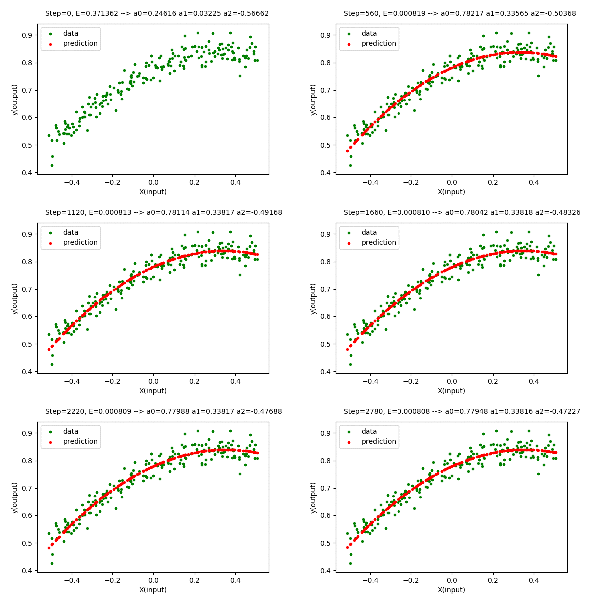
The value of the parameter matrix \(\boldsymbol{A}\) is very close to the optimal value of parameters.
\[\boldsymbol{A} = \begin{bmatrix} 0.77948 \\ 0.33816 \\ -0.47226 \end{bmatrix} \approx \begin{bmatrix} 0.77844 \\ 0.33815 \\ -0.46012 \end{bmatrix}\]The error value using gradient descent is \(0.00080786\) which is close to the minimum value of \(0.00080701\). Here, the method to determine the best degree of the polynomial is still the same. Everything is the same other than the way we find the optimal parameters.
Conclusion
In this post, we went through the basics of Polynomial Regression. We covered only the case of univariate polynomial regression using matrix inversion and gradient descent method. We can use more concise way of doing polynomial regression of a single variable as shown on this website. We can also perform polynomial regression on multivariate input. Check this math.stackexchange post to learn more.
Also, we covered additional concepts of Generalization, Bias-Variance Tradeoff, Model Selection, Non-Linear Curve Fitting, Hyperparameter Search, Gradient Descent with Matrices, etc. These concepts will be used further on upcoming blog posts to understand more topics.
There might be jumps while explaining the topics and may not be clear. There might arise further questions after reading all this. Also, there might be some errors that one may find. Please feel free to comment on the post, ask questions or give your feedback.
