Artificial Neural Network Back Then
Algorithm ·Artificial Neural Network (ANN) is one of the most popular Machine Learning Algorithm. As the name suggests, the algorithm tries to mimic the Biological Neural Network, i.e. the Brain. Although ANN does not function exactly like the brain, many features of ANN are inspired by the brain. To understand modern ANN algorithms, starting from the very beginning is a good idea. So, let us get into it starting from biological neurons first.
Python (Jupyter) Notebook used for this post and to generate GIFs is on this Github Repository. You can also run the Notebook on Google Collab
Biological Neuron and Neural Network
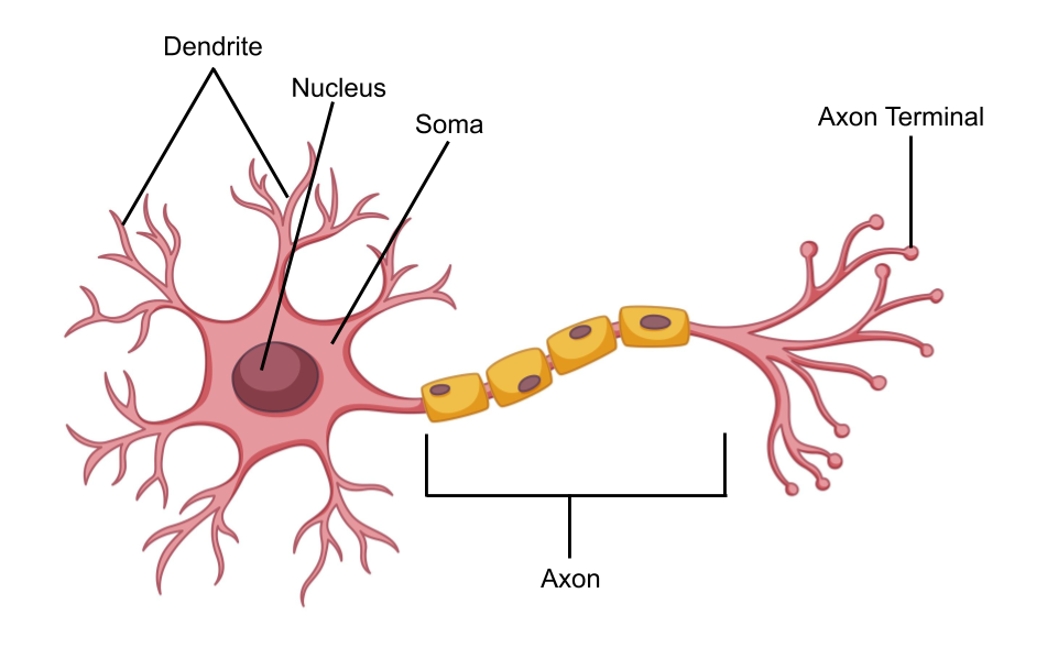
The term ‘Neuron’ was introduced in 1891. A neuron is the building block of the Nervous System (the Spinal cord and the Brain). The typical structure of the neuron is shown below.
Image Credit
A neuron is a biological signal processing and transmission unit. The working of a neuron can be explained sequentially.
Firstly, it receives an electrical signal from the dendrites (input). The dendrites are connected to axon terminal of other neurons. Secondly, it processes the input by measuring the total strength of the incoming signal. Incoming electrical signals all add up in soma. Finally, the neuron fires along its axon if the signal strength is large enough (output). The firing of a neuron (output signal) is received by other neurons connected to the axon terminal.
Collection of neurons interconnected with each other to form a network is called a Neural Network. If a neuron is represented by a Node and the connection between two neurons is represented by an Edge, the whole Neural Network can be represented by a Graph. There are generally three types of neurons. Sensory Neurons, which receive input from the world through sensory organs. Inner Neurons, which process the signal and store data. Motor Neurons, which control the muscles and glands.

This simple working mechanism of a single neuron combined with a large number of neurons (86 billion neurons) and even larger number of connections between them allows the Neural Network to do complicated functions such as language, vision and memory.
[Note: Neurons in the brain and spinal cord are of various types in their structure and functionality. Learn more at WyzSci: Youtube]
Although the working of the neuron was studied well, scientists did not know how neurons were responsible for learning and memory. Donald Hebb proposed a theory for learning in the synapse, summarized as “Neurons which fire together wire together”. This theory is called Hebb’s law and was used in 1954 for learning small Artificial Neural Network. This was one of the first learning rule for ANN.
The first step in modelling Biological Neural Network in the computer is to create a computational (or mathematical) model of the Neuron. This was done by McCulloch and Pitts in 1943.
McCulloch and Pitts model of a Neuron (1949)
Warren McCulloch and Walter Pitts modelled the first artificial neuron inspired from the biological neuron in 1943. This computational model of the Neuron is shown below.

The incoming signals to the neuron are modelled by input variables of the neuron. The dendrites are modelled by the weighted connection to the input variables. The cell soma is modelled by the weighted sum of the inputs. The output signal (axon firing) is given by the activation function (threshold) which outputs “1” if the weighted sum is above zero and outputs “0” otherwise.
This can be represented mathematically as:
\[\begin{align*} z &= w_0x_0 + w_1x_1 + w_2x_2 + \cdots + w_Nx_N\\ &= \sum_{i=0}^N w_ix_i \tag{1}\\ y &= \begin{cases} 1 &\text{if \(z>0\)}\\ 0 &\text{otherwise} \end{cases} \tag{2} \end{align*}\]Where,
\(x_i\) is the \(i^{th}\) input variable,
\(w_i\) is the corresponding weight to the input,
\(N\) is the total number of input variables,
\(y\) is the output of the Neuron.
Although this model of Artificial Neuron could be used to model [boolean functions] or [binary classifiers], there was no learning algorithm for it. The value of weights could still be found by using random search or grid search method (as discussed in Linear Regression). The goal of the search is to find values resulting in minimum error.
Let us use random search to find weights for OR Gate boolean function. For OR Gate there are two input variables (\(x_1\), \(x_2\)) and one output variable (\(t\)). The error of the function can be measured as follows.
\[E = \sum_{i=0}^N |y_i - t_i|\]Where,
\(y_i\) is the output of \(i^{th}\) input data,
\(t_i\) is the desired output (target) of \(i^{th}\) input data,
After searching, there were multiple values of \(w_1, w_2, w_3\) that gave minimum \(E\). One of the solutions has value \(w_1=-0.386, \,w_2=0.984, \,w_3=0.835\) and \(E=0\).
The function has 2 input variables (\(x_1\), \(x_2\)) and one output variable \(y\). This can be plotted in 3D graph as follows.
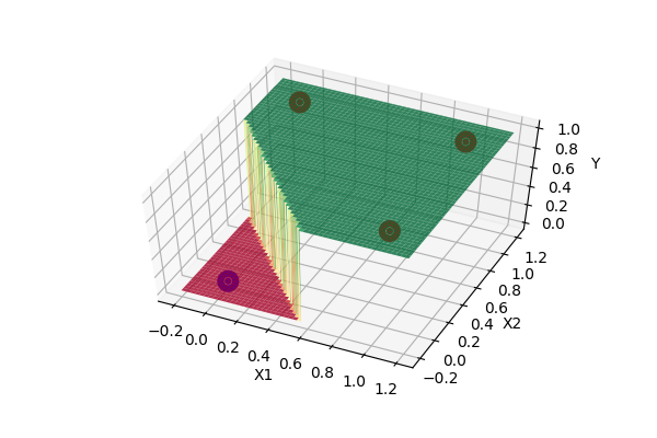
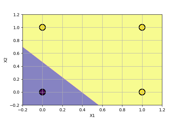
The function has two possible output values, i.e. \(y=0\) or \(y=1\). The 3D plot can be simplified into a 2D plot using color as output. In our case, yellow=”1” and blue=”0”. The 2D plot is as follows.
Hebbian Learning (1954)
Hebbian Learning theory was used by Farley and Wesley A. Clark to simulate Hebbian Network. Hebbian Network McCulloh and Pitts model of Neuron with Hebbian learning rule.
The goal of this rule is to strengthen the connection (increase the weight of the input) if the signal values are same, and weaken the connection if signal values different (decrease the weight of the input).
The Hebbian Network was used to model basic logic gates which use TRUE(1) and FALSE(-1) as input and output signals and real number for weights.
The Hebbian learning rule can be written mathematically as:
For each data point (i):
\[w_{n(new)} = w_{n(old)} + x_n^i.t^i\]Where,
\(x_n^i\) is the \(n^{th}\) input variable for \(i^{th}\) data point
\(w_{n(old)}\) is the previous weight.
\(w_{n(new)}\) is the updated weight.
\(x_n^i.t^i\) is the change in weight that takes value 1 if x and t are the same and -1 if different.
This algorithm was used to learn basic logic gates successfully. The model inspired by biological neuron was learned using learning theory of neurons. Great!!
Let us learn AND Gate with this algorithm. The truth table for AND Gate as follows:
\[\begin{vmatrix} \boldsymbol{x_1} \\ -1\\ -1\\ 1 \\ 1 \\ \end{vmatrix} \hspace{-2.5mm} \begin{vmatrix} \boldsymbol{x_2} \\ -1\\ 1\\ -1 \\ 1 \\ \end{vmatrix} \hspace{-2.5mm} \begin{vmatrix} \boldsymbol{t} \\ -1\\ -1\\ -1 \\ 1 \\ \end{vmatrix}\]The learning process can be visualized as follows.
We can see that the Network has learned AND boolean function. Same can be done for OR, NOT, NAND and NOR gates.
Although Hebbian learning successfully learned basic logic gates, it was unstable for many other examples. It had little mathematical foundation supporting the algorithm.
Perceptron and Perceptron Learning Rule (1958)
Perceptron was invented by Frank Rosenblatt at Cornell Aeronautical Laboratory in 1958. It was the actual implementation of the algorithm in the electro-mechanical device.
Perceptron came with its own learning rule called Perceptron Learning Rule (PLR). It had a mathematical foundation for the working of its algorithm. It used a Neural Network model similar to McClluoh and Pitts.
The algorithm for training Perceptron is shown below.
- Initialize all weights to zero (or small random value)
- Randomly select one of the data points \((\boldsymbol{x})\) from the dataset.
- Compute the output of the neuron as:
-
Update the parameters (weights) according to PLR as:
\(w_{i(new)} = w_{i(old)} + \alpha (t-y).x_{i}\)
Where,
\(\alpha\) is the learning rate in range [0, 1],
\(y\) is the output for given input and
\(t\) is the corresponding target value -
Repeat step 2, 3 and 4 until a certain step or until error E < threshold.
We can see in the update step (learning rule), the weights are changed if the output is wrong and not changed if the output is correct.
Let us use Perceptron and PLR to learn to classify the following data.

The yellow dots and blue dots denote two different class of data points. Our goal is to find parameters of Perceptron that successfully classify two classes of data points. We will use the learning rate (alpha) = 0.1. Following is the function learned by the algorithm at various steps of training.
Perceptron algorithm has found a solution for given data points. It can also be shown that it can also model basic boolean function, i.e. AND, OR, NOT Gates.
The problem with Perceptron is that it cannot find a solution (converge) if the data points are not linearly separable. It cannot model XOR Gate (XOR function is not linearly separable). We can try Perceptron with a noisy dataset and with XOR Gate as shown below.
We can see that the Perceptron algorithm does not converge for linearly inseparable data. In the noisy dataset, we can draw a straight line despite the noise to get the most probable decision boundary. In the case of XOR Gate, we cannot draw a straight line as the decision boundary. The problem cannot be solved by a linear classifier. This was pointed out by Marvin Minsky and Seymour Papert in their book Perceptron in 1969. They also showed that multiple layers of perceptron can be used to model XOR Gate and other linearly inseparable functions.
Also, Perceptrons could not model continuous real-valued functions. There was a need for better algorithms to solve all these problems.
Learn more about Perceptron Learning Rule and its convergence property PDF: here or Youtube: Cornell CS4780.
Multilayer Perceptron
In 1969, Minsky and Papert showed that Perceptron could not model function as simple as XOR Gate. They also proposed that multiple Perceptrons connected can model XOR Gate.
We know that Perceptron can model AND, OR, NAND Gates easily. We also know from boolean algebra that XOR Gate can be constructed from basic logic gates.
A XOR B = (A NAND B) AND (A OR B)
The above function can be modelled by Perceptrons as shown in the figure below.

The figure can be simplified removing obvious symbols as below.

This laid the basic idea for Multilayer Perceptron but at that time no learning algorithm could be used to train multiple layers at once.
It can be shown that MultiLayer Perceptron (MLP) can approximate any function up to arbitrary precision. This is called universal approximation theorem. This is the most important property of MLP. Multilayer Perceptron can be used to model any function (or any data).
Since there was no learning algorithm for MLP at that time, it was not much useful. This would change in upcoming years and Neural Network would continue to do complex AI tasks. The full history up to the current decade can be found at this site.
Checkout Youtube: CMU Deep Learning for more detail on Perceptron, MLP and Universal Approximation Theorem.
Conclusion
This post includes the history of the development of Artificial Neural Network, starting from understanding of biological neuron to algorithmic development and mathematical modelling of Universal Function Aprroximator. We have covered the capability of the algorithms as well as their limitations which needed to be overcome to build more complex AI systems. We have also covered the basic structure of the Neuron and its working, Hebbian theory, Perceptron and Multilayer Perceptron along with indirect coverage of classification using Neural Networks.
Please feel free to comment on the post, ask questions or give feedback.