Dynamic 1D Piecewise Linear Spline Function Approx.
Research, Algorithm ·In previous posts, we covered the fundamentals of Linear Regression for fitting a line to data, non-linear function approximation with Polynomial Function as well as MultiLayer Perceptron. We also covered some content on Piecewise Functions - Linear Spline, MLP and Decision Tree and conversion between them in 1D in a video. In this post, we dive into how we can use linear spline for function approximation, dive into the mathematical details and make it dynamic by adjusting the number of break points (or control points or pieces) using heuristics.
I am excited to share this with you as it was one of the initial works I took upon myself, did maths, implemented it and it worked. It provided me with the initial motivation to pursue research. Although this is a small work, it provided a foundation for my later works. You can check out my repository during the development - library, spline-1d and spline-nd. I have shared the notebook used for developing visualizations in this post at github. Hope you are excited too! Let’s get started!
Piecewise Linear Spline
There are various types of splines as shown in Figure above. We are concerned only about linear splines which creates PieceWise Linear Function (PWLF). For simplicity, we would start with just one piece, derive the gradients, and later extend to multiple pieces.
A piecewise linear function with only 1 piece connecting points \((x_0, y_0)\) and \((x_1, y_1)\) can be defined as follows:
\[\begin{align*} y = f(x) &= \begin{cases} \frac{y_1-y_0}{x_1-x_0}(x-x_0)+y_0 &\text{if \(x_0 \leq x < x_1\)}\\ \end{cases} \end{align*}\]Here, \(y\) is the prediction/output. If we consider \(t\) to be the target output, then the MSE loss (\(E\)) can be defined as
\[E=\frac{1}{2n} \sum_{i=0}^{n-1} (y^{(i)} - t^{(i)})^2\]where, \(t^{(i)}\) is the target of \(i^{th}\) element in the dataset containing \(n\) items. The graident with respect to output is \(\frac{dE}{dy^{(i)}} = y^{(i)} - t^{(i)}\). For simplicity of understanding, we only take one sample \(x\), its output \(y=f(x)\), target \(t\), then the gradient with respect to \(y\) is given as:
\[\frac{dE}{dy} = \Delta{y} = y - t\] \[\Delta{y} = \begin{cases} \frac{y_1-y_0}{x_1-x_0}(x-x_0)+y_0 - t &\text{if \(x_0 \leq x < x_1\)}\\ \end{cases}\]We can calculate the gradient with respect to the parameters \(x_0, y_0, x_1, y_1\) using the chain rule.
\[\begin{align*} \Delta{y_0} &= \frac{dE}{dy_0} = \frac{dE}{dy} \frac{dy}{dy_0} \\ &= \Delta{y}(1-\frac{x-x_0}{x_1-x_0}) \\ \Delta{y_1} &= \frac{dE}{dy_1} = \frac{dE}{dy} \frac{dy}{dy_1} \\ &= \Delta{y}\frac{x-x_0}{x_1-x_0} \\ \Delta{x_0} &= \frac{dE}{dx_0} = \frac{dE}{dy} \frac{dy}{dx_0} \\ &= \Delta{y}(y_1-y_0)\frac{x-x_1}{(x_1-x_0)^2} \\ \Delta{x_1} &= \frac{dE}{dx_1} = \frac{dE}{dy} \frac{dy}{dx_1} \\ &= -\Delta{y}(y_1-y_0)\frac{x-x_0}{(x_1-x_0)^2} \\ \end{align*}\]We leave the details of this derivation as an excercise to the reader. If you can’t find the solution, I am happy to help.
Combining multiple pieces of linear spline
We can define the Piecewise Linear Function for multiple pieces: \(m+1\) control points (indexed \(0\) to \(m\)) produce \(m\) linear pieces. We already defined the forward function and derived backward gradients for only 1 piece with 2 control points. Now we extend the forward function for multiple pieces.
\[\begin{align*} y = f(x) &= \begin{cases} \frac{y_1-y_0}{x_1-x_0}(x-x_0)+y_0 &\text{if \(x_0 \leq x < x_1\)}\\ \frac{y_2-y_1}{x_2-x_1}(x-x_1)+y_1 &\text{if \(x_1 \leq x < x_2\)}\\ \vdots \\ \frac{y_{i+1}-y_{i}}{x_{i+1}-x_{i}}(x-x_{i})+y_{i} &\text{if \(x_{i-1} \leq x < x_{i}\)}\\ \end{cases} \end{align*}\]For simplicity, we refer to the pieces in terms of index of the piece or control points rather than input range as follows:
\[\begin{align*} y = f(x) &= \begin{cases} \frac{y_{i+1}-y_{i}}{x_{i+1}-x_{i}}(x-x_{i})+y_{i} &\text{if \(0\leq i \leq m-1\)}\\ \end{cases} \end{align*}\]When working with multiple pieces, we want to differentiate the \(\Delta y\) gradients from multiple pieces. We use subscript to denote the \(i^{th}\) piece connecting \(i^{th}\) and \(i+1^{th}\) control points as shown below.
\[\begin{align*} \frac{dE}{dy} = \Delta{y} &= \begin{cases} \frac{y_{i+1}-y_i}{x_{i+1}-x_i}(x-x_i)+y_i - t &\text{if \(0\leq i \leq m-1\)}\\ \end{cases} \\ \Delta{y} &= \begin{cases} \Delta y_{(i,i+1)} &\text{if \(0\leq i \leq m-1\)}\\ \end{cases} \end{align*}\]When it comes to computing the gradient, a single break point is shared by 2 pieces, hence the gradient of the shared piece is the sum of the gradient from both pieces. This results in a gradient of parameters as defined below:
\[\begin{align*} \frac{dE}{dy_i} &= \begin{cases} (1-\frac{x-x_i}{x_{i+1}-x_i})\Delta y_{(i,i+1)} &\text{if $i=0$}\\ (1-\frac{x-x_i}{x_{i+1}-x_i})\Delta y_{(i,i+1)} + (\frac{x-x_{i-1}}{x_{i}-x_{i-1}})\Delta y_{(i-1,i)} &\text{if $0<i<m$}\\ (\frac{x-x_{i-1}}{x_{i}-x_{i-1}})\Delta y_{(i-1,i)} &\text{if $i=m$}\\ \end{cases} \end{align*}\]Similarly, for gradient with respect to x parametes:
\[\begin{align*} \frac{dE}{dx_i} &= \begin{cases} \frac{(y_{i+1}-y_i)(x-x_{i+1})\Delta y_{(i,i+1)}}{(x_{i+1}-x_i)^2} &\text{if $i=0$}\\ \frac{(y_{i+1}-y_i)(x-x_{i+1})\Delta y_{(i,i+1)}}{(x_{i+1}-x_i)^2} - \frac{(y_i-y_{i-1})(x-x_{i-1})\Delta y_{(i-1,i)}}{(x_i-x_{i-1})^2} &\text{if $0<i<m$}\\ - \frac{(y_i-y_{i-1})(x-x_{i-1})\Delta y_{(i-1,i)}}{(x_i-x_{i-1})^2} &\text{if $i=m$}\\ \end{cases} \end{align*}\]I have written the equation in compact and generalized it to all indexes. If this is difficult for you, please try to derive using 2 pieces for which there are 3 control points.
Visualizing Fitting of function
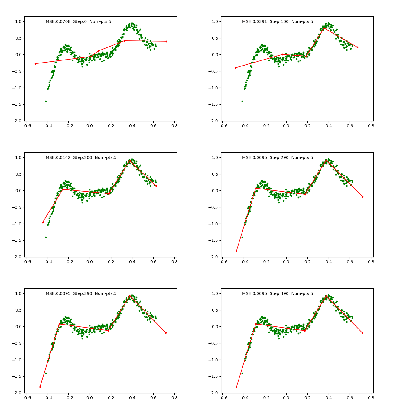
We simply use SGD optimizer on the parameters and train it on a toy 1D regression problem as we did for earlier algorithms. The training is done with 4 pieces (5 break points), which can be observed as follows:

Problems observed and solved.
We faced multiple problems during the training experiments and used different tricks to make it more stable. Next, we go into the problems and how we use heuristics to fix the problems to create a robust 1D PWLF.
1. Limit edge break points to be outside input samples: The first problem that we faced is that when the control points are updated, the x-value of the edge control points lies inside the dataset, i.e. some data points do not lie inside the spline. Hence, we check if the first(\(i=0\)) and last control point(\(i=m\)) are outside the data range and enforce it every update.
2. Internal break point outside data points: In many cases, the multiple break points lie outside the region containing data samples. This creates unused pieces which are not important for prediction, rather, we detect if there are pieces with no data points and remove them.
3. Combine linear pieces (or remove unuseful break point): There are cases when the 3 consecutive break points create an almost linear spline (with very small non-linearity). In the figure below, we can observe that the spline \(acb\) is highly non-linear, however, the spline \(adb\) has little non-linearity. In such a case, we can remove the control point \(d\) and directly connect \(ab\).
The amount of non-linearity can be defined using the area of the triangle defined by 3 consecutive points. If the area is lower than a certain threshold (0.01 in below experiments), then we remove such control points.
4. Combine very small pieces (or remove close break point): If the x-coordinate of a control point is very close to another control point, then such a piece should be removed, it might cause a piece to jump abruptly and also under-utilize the control points. We simply set a threshold (0.001 for the below experiments) for the gap between pieces, below which one of the control points is removed.
5. Add new piece (or break point): If the function is not approximating the dataset properly, we may have a lower number of splines than required to perfectly fit the dataset. Hence, we need a mechanism to add a new piece or a break point to the function. In our code, we simply search for a piece with the highest error, and if the error is greater than the threshold (0.0001 for the below experiments), we proceed to add a piece at some random control point inside the bounding control points. We initialize the y-value of the point to be the output of the spline itself, hence the function is not changed even after addition, however, now it can be optimized to fit the dataset better.
Dynamic 1D Piecewise Function
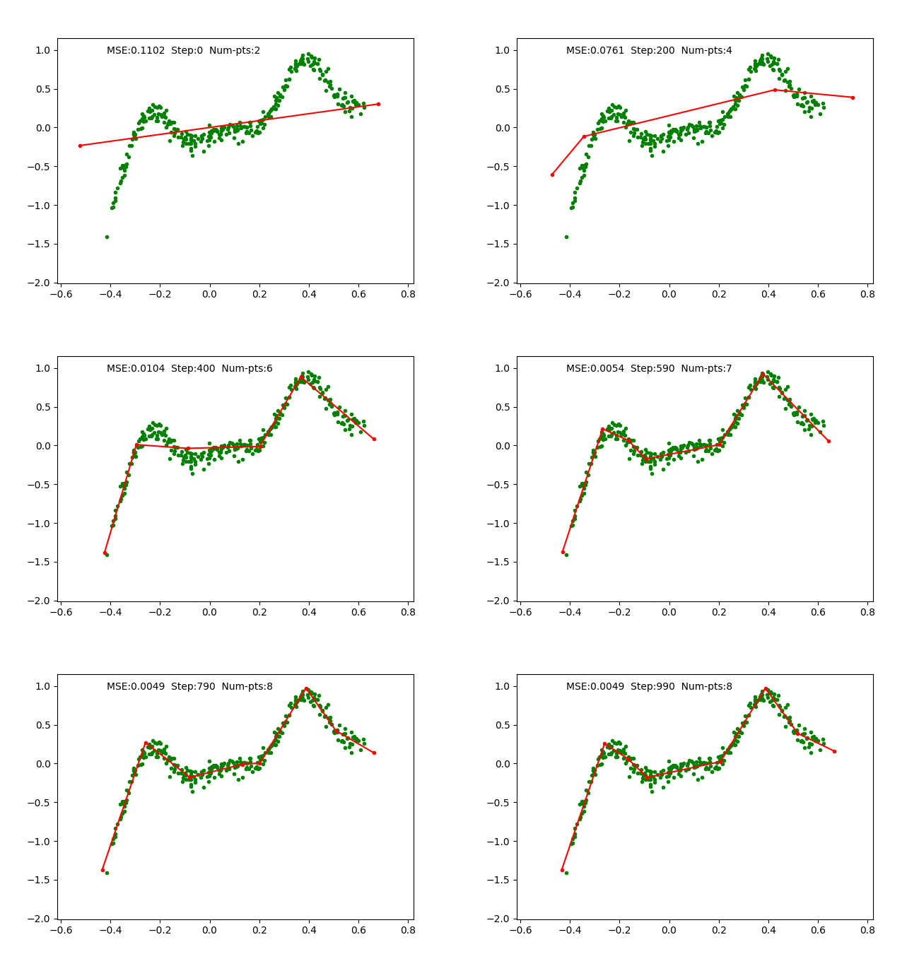
Iteratively fixing PWLF, adding and removing break points allows us to approximate a 1D function with high non-linearity starting just with 1 piece (or a linear function). We can visualize the function approximation as follows, where we maintain the PWLF problems every N (=100) steps.

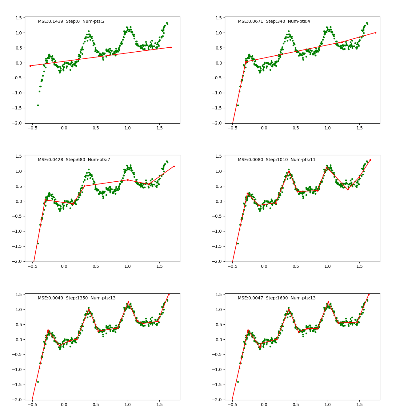
We also visualize a more non-linear function extending to larger range as follows:

The big limitation of our work is that this is just limited to 1D, i.e. it does not generalize to higher dimensions. We tried to replace away linear connection in MLP with PWLF and it works for small networks, however, it seems to get stuck at local minima for a large number of connections. Moreover, our implementation is not highly optimized, hence works slowly when the connections increase.
Exploring PWLF on nD
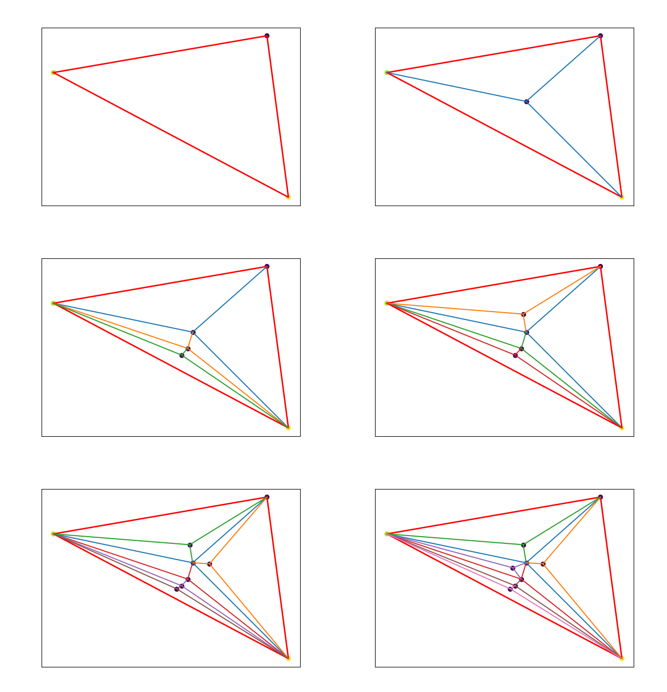
We may generalize a piece (a line in 1D) to higher dimensions: triangle in 2D, tetrahedron in 3D and so on (called simplex). The figure below shows how I tried to break each triangle into subparts for PWLF in 2D.

Although I couldn’t make it work for regression and classification problems and my implementation is not efficient. I believe triangular mesh or mesh with simplexes (simplicial complex) could work for regression and classification in high dimensions. Moreover, simplices are very important in 3D graphics, convex hulls, topology and more. Hope you study additional resources on this.
Conclusion
In this post, we started by defining a single piece, deriving its gradients, and extending it to multiple pieces to create 1D PWLF. We later solved multiple problems to create a dynamic PWLF which could adjust its capacity (or the number of break points) according to the complexity of the input data.
Moreover, the way the piecewise linear spline function is computed is very intuitive and can create a highly non-linear function with each break point having a local effect on the overall function.
This simple research on PWLF and dynamic function came to huge aid in my future works which I will cover in later posts.
