Perceptron to Deep-Neural-Network
Algorithm ·Neural Network is one of the most versatile Machine learning Algorithms. It has come a long way from early methods such as Perceptron. Many people jump directly into Deep Learning and face a problem understanding what exactly the algorithm is doing. It is useful to ignore the details by calling it a black box that just works. It is more useful to understand the details of its working for research and tinkering purpose.
In this post, we will follow a gradual path from the earliest algorithm (Perceptron) to Deep Neural Networks. This post is based on my journey to connect primitive Perceptron Algorithm to the modern Deep Neural Network Algorithms.
This post is organized into four parts:
1. Improving on Perceptron Algorithm
2. Non-Linear Regression with Backpropagation
3. Multilayer Perceptron (1 hidden layer)
4. Deep Neural Networks
Python (Jupyter) Notebook used for this post and to generate GIFs is on this Github Repository. You can also run the Notebook on Google Collab
This is a lengthy post; brace yourself. Let us begin our journey.
Improving on Perceptron algorithm
We have covered a lot about Perceptron on the previous post. The algorithm is unstable when classifying data with noisy decision boundary points. Although we can manually draw a decision boundary to classify the points best, the Perceptron is not able to do so. The algorithm is unstable as can be seen in the figure below.
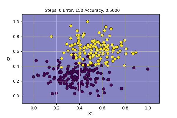
We can see that the algorithm changes the decision boundary for each data point with an error. Since we will always have some error with such noisy dataset, the algorithm does not converge (find a final solution).
We can also see the Accuracy and Error keeps fluctuating. This is useful to compare with other methods.
We can guess that the fluctuations are due to optimizing for one data point at a time. What will happen if we update the parameters of the function for the whole dataset?
Training Perceptron on full batch Dataset
We can train the Perceptron with the gradient of the parameter for the whole batch as follows:
- For each \((\boldsymbol{x_i}, y_i)\) in the dataset (\(\boldsymbol{X}, \boldsymbol{y}\)), compute the output:
\(\qquad \hat{y_i} = f_{step}(\boldsymbol{x_i^T}.\boldsymbol{w})\) - Compute the gradient for the weights:
\(\qquad \Delta \boldsymbol{w} = \frac{1}{N} \sum_{i=0}^{N-1} (\hat{y_i} - y_i)\boldsymbol{x_i}\) - Update the parameters:
\(\qquad \boldsymbol{w} = \boldsymbol{w} - \Delta \boldsymbol{w}\) - Repeat step 1 to 3 for \(M\) steps.
Where,
\(f_{step}\) is the step function,
\(\boldsymbol{x_i} \in \mathbb{R}^{3}\) is the \(i^{th}\) input vector,
\(\boldsymbol{w} \in \mathbb{R}^{3}\) is the weight vector,
\(N\) is the number of data points.
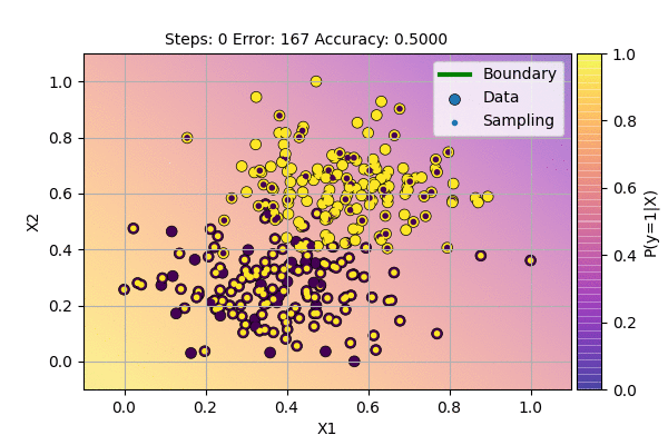
We can visualize the learning of the Perceptron with batch update as follows.

We can see that the decision boundary is more stable and also gives more stable accuracy. It seems that we can do better learning using the batch update. Still, the problem is not fully solved. We may decrease the learning rate over time to decrease the change in decision boundary.
We can again guess what the problem is due to. The dataset does not have a clean decision boundary to make 100% sure classification. The points making error are equally valid data points as the correctly classified data points. We can use fuzzy decision boundary, around which the classification is not certain.
We can incorporate probability into the classification to make room for uncertain(opposing) data points.
Training Perceptron with Probability
There exists a function that can give the probability of the data points belonging to class ‘1’. It is called the logistic sigmoid function.

The logistic sigmoid function is given by:
\[\begin{align} \hat{y} &= \sigma(x) \\ & = \frac{1}{1+e^{-x}} \tag{1} \end{align}\]Probability 1, \((\hat{y} = 1)\), means that the data point belongs to class ‘1’ and probability 0 means that the data point does not belong to class ‘1’ (hence belongs to class ‘0’). The probability of 0.5 means the data point has 50/50 chance to be in class ‘0’ or class ‘1’. Hence this point can be regarded as the decision boundary. We can use other threshold values for the decision boundary as well. In medical application, if the classifier predicts the probability of having cancer, we might want probability > 0.7 to be more certain about the diagnosis.
Although we formulate the problem in terms of probability, we don’t know the learning required for probability values. One solution is to sample from probability to make a hard decision. This will predict noisy output around the decision boundary. The algorithm can then be simply trained as a (noisy) Perceptron.
The training Algorithm for Noisy Perceptron is as follows.
- For each \((\boldsymbol{x_i}, y_i)\) in the dataset (\(\boldsymbol{X}, \boldsymbol{y}\)), compute the output:
\(\qquad z_i = P(y=1|\boldsymbol{x_i}) = \sigma (\boldsymbol{x_i^T}.\boldsymbol{w})\)
\(\qquad \hat{y_i} \sim Bernoulli(z_i)\) - Compute the gradient for the weights:
\(\qquad \Delta \boldsymbol{w} = \frac{1}{N} \sum_{i=0}^{N-1} (\hat{y_i} - y_i).\boldsymbol{x_i}\) - Update the parameters:
\(\qquad \boldsymbol{w} = \boldsymbol{w} - \Delta \boldsymbol{w}\) - Repeat step 1 to 3 for \(M\) steps.
Where,
\(\sigma (x)\) is the sigmoid function,
\(z_i \sim Bernoulli(\hat{y})\) is sampling from Bernoulli distribution with probability \(\hat{y}\).
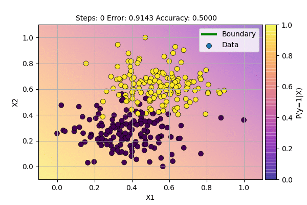
We can visualize the Algorithm at the action as follows.
This is even better because we get slightly higher accuracy even with noise in the system. During the testing phase, we use a threshold function according to the required probability. Here, we use Bernoulli Distribution for sampling. This is because we have two possible cases: \(y=1\) (Success) and \(y=0\) (Failure). The point with probability 0.5 will be sampled as class 0 half of the time and as class 1 half of the time. But with this method, the decision boundary will never be stable. We can lower the learning rate to force it to be stable, but we want the algorithm itself to find stable decision boundary.
The parameters of a probability distribution can be estimated by using Maximum Likelihood Estimation (MLE) method. In statistics, maximum likelihood estimation is a method of estimating the parameters of a probability distribution by maximizing a likelihood function, so that under the assumed statistical model the observed data is most probable. This method will be discussed in the next topic. You may skip the derivation of Logistic Regression
Logistic Regression (Derivation)
Suppose that our data came by sampling from some population of data points. If we assume that the data was generated by some underlying probability distribution, then we may try to estimate parameters of the distribution.
Suppose that \(y\) came by sampling from some probability distribution with \(\boldsymbol{x}\) as input(independent variable) and \(y\) as outcome.
Since we have two classes as output, we can assume that the data points were sampled from Bernoulli distribution.
\[y \sim Bernoulli(p)\]Here, \(p\) is the underlying probability distribution over \(\boldsymbol{x}\) that determines the outcome \(y\). So, we can write,
\[p=P(y=1|\boldsymbol{x})\]Our goal is to model the \(p\) given only the observation/dataset (\(\boldsymbol{X}, \boldsymbol{y}\)).
The Bernoulli distribution can be modelled by a simple function as follows.
Here, \(\sigma (z)\) is the sigmoid function given by equation (1).
Similarly,
The equations (3) and (4) can be written in a single formula as,
\[P(y) = \hat{y}^y (1-\hat{y})^{(1-y)} \tag{4}\]Our goal is to get highest probability,\(P(y)=1\)(correct prediction),for all \(y\) in the dataset with our model \(\hat{y}\). We may not get highest probability but we can surely try our best to maximize it. The probability of all the data points to have come from the modeled distribution (equation 4) is called the likelihood. Hence, we want to maximize the likelihood of the above function.
For each data point \(\boldsymbol{x_i}\),
\[\begin{align} z_i &= \boldsymbol{x_i^T}.\boldsymbol{w} \tag{5}\\ \hat{y_i} &= \sigma (z_i) \\ &= \frac{1}{1+e^{-z_i}} \tag{6}\\ \end{align}\]The likelihood function of \(P(y_i|\boldsymbol{x_i};\boldsymbol{w})\) for all (\(\boldsymbol{x_i}, y_i\)) in dataset \((\boldsymbol{X}, \boldsymbol{y})\) is as follows:
\[\begin{align} L(\boldsymbol{y}|\boldsymbol{X}; \boldsymbol{w}) &= P(\boldsymbol{y}|\boldsymbol{X};\boldsymbol{w})\\ &= \prod_{i=0}^{N-1} P(y_i|\boldsymbol{x_i};\boldsymbol{w})\\ &= \prod_{i=0}^{N-1} \hat{y_i}^{y_{i}} (1-\hat{y_i})^{(1-y_i)}\\ \end{align}\]Since our goal is to maximize the likelihood function \(L(\boldsymbol{y}|\boldsymbol{X};\boldsymbol{w})\) , we will use calculus for this.
\[\begin{align} \boldsymbol{w}^* &= arg\max_{\boldsymbol{w}} L(\boldsymbol{y}|\boldsymbol{X};\boldsymbol{w})\\ &= arg\min_{\boldsymbol{w}} - \log L(\boldsymbol{y}|\boldsymbol{X};\boldsymbol{w}) \end{align}\]Maximizing a function is equivalent to minimizing the negative log of the function. We can expand the Neagtive-Log-Likelihood function as:
\[\begin{align} -\log L(\boldsymbol{y}|\boldsymbol{X};\boldsymbol{w}) &= - \sum_{i=0}^{N-1} \log(\hat{y_i}^{y_i}) + \log((1-\hat{y_i})^{(1-y_{i})}) \\ &= - \sum_{i=0}^{N-1} y_i \log\hat{y_i} + (1-y_{i}) \log(1-\hat{y_i}) \tag{7} \end{align}\]Since we have \(N\) data points, we can normalize the Negative-Log-Likelihood (NLL) function by N and still have the same minimization objective. This NLL function is also called a Binary-Cross-Entropy function. It measures the discrepancy between actual value \((y_i)\) and modelled value \((\hat{y_i})\). In case of binary classification, \(y_i \in \{0, 1\}\) but \(\hat{y_i}\) can take any value in range \((0,1)\). It can be taken as the Error function (E) of the model.
If we take \(E_i = - y_i \log\hat{y_i} - (1-y_{i}) \log(1-\hat{y_i})\) as error for individual data points then,
\[\begin{align} E &= -\frac{1}{N} \log L(\boldsymbol{y}|\boldsymbol{X};\boldsymbol{w}) \\ &= -\frac{1}{N} \sum_{i=0}^{N-1} y_i \log\hat{y_i} + (1-y_{i}) \log(1-\hat{y_i}) \tag{8}\\ &= \frac{1}{N} \sum_{i=0}^{N-1} E_i \end{align}\]Minimizing the Binary-Cross-Entropy (equation 8), gives us the parameters of the model. But unfortunately, there is no analytical solution to this. We need to find parameters using iterative method such as Gradient Descent.
Using Gradient Descent to minimize the Error
The gradient of the Error(E) with respect to (w.r.t) the parameter \(\boldsymbol{w}\), i.e, \(\frac{dE}{d\boldsymbol{w}}\), can be used to minimize the Error function.
\[\frac{dE}{d\boldsymbol{w}} = \frac{1}{N}\sum_{i=0}^{N} \frac{dE_i}{d\boldsymbol{w}} \tag{9}\]We can expand the derrivative \(\frac{dE_i}{d\boldsymbol{w}}\) as follows.
\[\begin{align} \frac{dE_i}{dz_i} &= \frac{dE_i}{d\hat{y_i}}.\frac{d\hat{y_i}}{dz_i} \\ and, \frac{dE_i}{d\boldsymbol{w}} &= \frac{dE_i}{dz_i}.\frac{dz_i}{d\boldsymbol{w}} \\ &= \frac{dE_i}{d\hat{y_i}}.\frac{d\hat{y_i}}{dz_i}.\frac{dz_i}{d\boldsymbol{w}} \tag{10} \end{align}\]This above method of expanding the partial derrivatives is called the chain rule. It is called backpropagation in Machine Learning. It is used here to propagate gradient of the Error function \((E)\) from \(\hat{y_i}\) to \(z_i\) to \(\boldsymbol{w}\).
Let us solve for the individual derivative term in equation (10).
\[\begin{align} \frac{dE_i}{d\hat{y_i}} &= \frac{d(- y_i \log\hat{y_i} - (1-y_{i}) \log(1-\hat{y_i}))}{d\hat{y_i}}\\ &= -\frac{y_i}{\hat{y_i}} + \frac{1-y_{i}}{1-\hat{y_i}} \\ &= \frac{y_i - \hat{y_i}}{\hat{y_i}(1-\hat{y_i})} \tag{11} \\ \frac{d\hat{y_i}}{dz_i} &= \frac{d(\frac{1}{1+e^{-z_i}})}{dz_i}\\ &= \frac{-1}{(1+e^{-z_i})^2}.e^{-z_i}.-1 \\ &= \frac{1}{1+e^{-z_i}}.(1-\frac{1}{1+e^{-z_i}}) \\ &= \hat{y_i}(1-\hat{y_i}) \tag{12} \\ \frac{dz_i}{d\boldsymbol{w}} &= \frac{d(\boldsymbol{w}.\boldsymbol{x_i})}{dz_i}\\ &= \boldsymbol{x_i} \tag{13} \\ \end{align}\]Substituting equation 11, 12, 13 in equation (10), we get:
\[\begin{align} \frac{dE}{d\boldsymbol{w}} &= \frac{1}{N}\sum_{i=0}^{N} \frac{y_i - \hat{y_i}}{\hat{y_i}(1-\hat{y_i})}. \hat{y_i}(1-\hat{y_i}) . \boldsymbol{x_i} \\ \Delta \boldsymbol{w}&= \frac{1}{N}\sum_{i=0}^{N} (y_i - \hat{y_i}).\boldsymbol{x_i} \tag{14} \end{align}\]This is the gradient of weights for training the Logistic Regression. This can be written in Matrix form for whole dataset as follows.
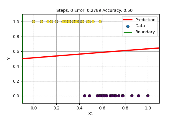
\[\Delta \boldsymbol{w} = \frac{1}{N} \boldsymbol{X^T}.(\boldsymbol{\hat{y}} - \boldsymbol{y})\]Training Logistic Regression (Binary Classifier)
The gradient for Logistic Regression looks similar to the Perceptron Learning Algorithm but with sigmoid activation function. The training Algorithm for Logistic Regression is as follows.
- For each \((\boldsymbol{x_i}, y_i)\) in the dataset (\(\boldsymbol{X}, \boldsymbol{y}\)), compute the output:
\(\qquad \hat{y_i} = P(y=1|\boldsymbol{x_i}) = \sigma (\boldsymbol{x_i^T}.\boldsymbol{w})\) - Compute the gradient for the weights:
\(\qquad \Delta \boldsymbol{w} = \frac{1}{N} \sum_{i=0}^{N-1} (\hat{y_i} - y_i)\boldsymbol{x_i}\) - Update the parameters:
\(\qquad \boldsymbol{w} = \boldsymbol{w} - \Delta \boldsymbol{w}\) - Repeat step 1 to 3 for \(M\) steps.
Let us use this algorithm to classify our data.
This is even better than the sampling case. We are still using the same model but achieve faster convergence and stable decision boundary. The decision boundary is stable but the gradient never reaches zero because there is error around decision boundary and sigmoid outputs are never exactly 0 or 1.
We have solved one of the problems of the perceptron, working with noisy decision boundary. The other problem of linearly-inseparable data like XOR gate is still not solved. We will visit that later.
We have seen that the perceptron and logistic regression uses linear transformation followed by non-linearity (step function in Perceptron, sigmoid function in Logistic Regression). Another problem with perceptron was it could not produce continuous (Real-valued) output. We have used sigmoid to produce continuous value already.
Linear Regression, Perceptron, Logistic Regression all look too similar. Can we make a general model from all these?
Yes, we can. All these functions have Linear-Transformation followed by Activation Function and Gradient is computed to minimize/maximize some objective function.

Note: Using constant input \(x_0 = 1\) with weight \(w_0\) is equivalent to having no constant input but with bias term \(b\) added to the weighted sum
If we use the linear activation function (\(f(x) = x\)) with \(E(\hat{y}, y)\) = MSE, we get Linear regression. With \(f(x) = step(x)\) and \(E(\hat{y}, y)\) = Hinge Loss, we get Perceptron. Similarly, \(f(x) = \sigma(x)\) and \(E(\hat{y}, y)\) = Binary Cross Entropy, we get Logistic Regression.
A question arises, what if we train with \(f(x)= \sigma(x)\) and \(E(\hat{y}, y)\) = MSE. This is trying to solve the classification problem with a regression loss function. Let us try this to classify 1D data with Logistic Regression and with single layer Sigmoid-Neural Network.
The single layer NN with sigmoid activation function works just fine but it updates slowly. On what other data can we use sigmoid based non-Linear regression?
Let us make an S-shaped curve with some noise. We can perform Non-linear regression as follows.
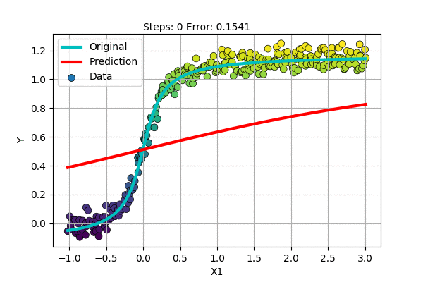
It does well and seems better than fitting a line. But still, if the top portion moved a little higher, it would have been perfect.
Also, it seems that we need a special-shaped function for each dataset if we continue to follow this path. Polynomial Regression was much better than this, it was general.
We could improve on the regression by transforming data into higher dimension such as polynomial regression. The transformations generally include using a polynomial combination of variables. The variables \((x_1, x_2)\) can be transformed to \((x_1, x_2, x_1^2, x_2^2, x_1x_2, \dots )\) and use Linear Regression with these variables. This is another fantastic area to explore. These type of methods are called Kernel Methods and is widely used with SVMs. Check out solving XOR gate using single perceptron.
Non-Linear Regression with Backpropagation
While dealing with Non-Linear Regression problem as above, we are scaling the input with Weights (W), shifting using bias/intercept (b) and non-linear function (\(\mathbb{R} \to \mathbb{R}\)) to introduce non-linearity.
These functions have a specific property. The sigmoid always outputs in range (0, 1). If we have S-shaped data in range (1, 3), we cannot do the regression with sigmoid.
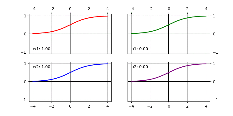
This can be improved by using additional variables to scale and shift the output.
\[z = f(\boldsymbol{x^T}.\boldsymbol{w_1} + b_1)\]We can scale by multiplying and shift by adding to the output of non-linear activation.
\[\hat{y} = f(zw_2 + b_2)\]
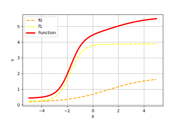
We can visualize the sigmoid based non-linear function after scaling and shifting as follows. It shows how the function changes when changing individual parameters. The default value used in the function below is \(w_1 = 1, b_1 = 0, w_2 = 1, b_2 = 0\).
We can compute the gradient easily using chain rule (aka Backpropagation).
[Reader can easily derive gradient for parameters \(W_1, b_1, W_2, b_2\) as an excercise]
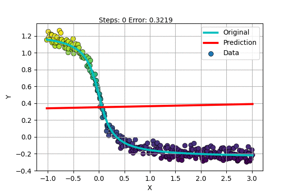
Let us try to fit an inverted S-shaped function with our new model.
But there are more complex functions and only some are S-shaped. What about the rest? Do we find a special function for each dataset?
We know that just like we operate on numbers, we can operate on functions. We can multiply, add and compose multiple functions. This generally results in more complex function than the individual functions.
Consider the following example.
\[\begin{align} y_1 &= 2 \log x \\ y_2 &= \cos x + 1 \\ y &= y_1+ y_2 \\ &= 2 \log x + \cos x + 1 \\ \end{align}\]Here, \(y\) is more complex function than \(y_1\) and \(y_2\)
Functions can be formed by adding (or multiplying or dividing) multiple functions. Adding two or more functions is called superposition of functions. Fourier Series is one of the greatest examples to demonstrate this property. It says that any periodic function can be composed by adding many weighted sine and cosine functions.
Similarly, we can create complex functions by adding scaled and shifted sigmoid functions. Let us add randomly generated functions to see how the superposition looks like.
We can see that adding more of the simple functions can generate more complex functions. It has been proven that such superposition of sigmoid functions can approximate any function. Check neuralnetworksanddeeplearning for graphical proof.
This exact method of constructing complex function using simple functions is what Multilayer Perceptron does.
Multilayer Perceptron
Let us define simple function discussed above as follows.
\[\begin{align} z^{(i)} &= f(\boldsymbol{x^T}.\boldsymbol{w_1}^{(i)} + b1^{(i)}) \\ \hat{y}^{(i)} &= w_2^{(i)}z^{(i)} + b_2^{(i)} \\ \end{align}\]The superposition of \(M\) such functions can be represented as:
\[\hat{y} = \hat{y}^{(0)} + \hat{y}^{(1)} + \dots + \hat{y}^{(M-1)}\]This can be represented in vector/matrix form as follows.
\[\begin{align} \boldsymbol{z^T} &= f(\boldsymbol{x^T}.\boldsymbol{W_1} + \boldsymbol{b1}) \\ \hat{y} &= \boldsymbol{z^T}.\boldsymbol{w_2} + b_2 \\ \end{align}\]Where,
\(\boldsymbol{W_1}= \begin{bmatrix} | &| &\dots &|\\ \boldsymbol{w_1}^{(0)} &\boldsymbol{w_1}^{(1)} &\dots &\boldsymbol{w_1}^{(M-1)}\\ | &| &\dots &| \end{bmatrix}\) \(\boldsymbol{b_1}= \begin{bmatrix} b_1^{(0)} \\ b_1^{(1)} \\ \vdots \\ b_1^{(M-1)} \end{bmatrix}\) \(\boldsymbol{w_2}= \begin{bmatrix} w_2^{(0)} \\ w_2^{(1)} \\ \vdots \\ w_2^{(M-1)} \end{bmatrix}\)
\[b_2=b_2^{(0)} + b_2^{(1)} + \dots + b_2^{(M-1)}\]Here,
\(\boldsymbol{x} \in \mathbb{R}^{I} ;\) \(\boldsymbol{W_1} \in \mathbb{R}^{I \times M} ;\) \(\boldsymbol{b_1} \in \mathbb{R}^{M};\) \(\boldsymbol{w_2} \in \mathbb{R}^{M};\) \(b_2 \in \mathbb{R} ;\)
\(\boldsymbol{z^T} \in \mathbb{R}^{M}\) denotes the row vector of hidden unit values.
The diagram representation of MLP with 2 inputs, 3 hidden units and one output is shown below.
![Fig: Multilayer Perceptron Architecture with configuration [2,3,1]](/assets/post_images/perceptron-to-dnn/nn-2-3-1.svg)
Let us train a Multilayer Perceptron with 5 hidden units to learn a non-linear curve (1D to 1D) as shown below.
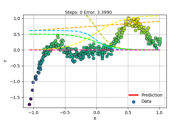
We can visualize the superposition of simple functions forming the compex curve as shown in the figure below.

MLP for multivariate output
We have only discussed the single-valued (scalar) output case. How do we perform Nonlinear Regression for multivariate output (vector output)? One simple idea is to use a different MLP’s for each variable as shown below.

This is equivalent to having all weights of upper hidden layers connecting \(y_1\) to be zero. And all weights connecting lower layers to \(y_0\) to be zero.
We can profit more if those weights are non-zero. We can model even more complex function if we use all hidden units. Hence, the hidden layer is shared for all output variables.

General Equation of Multilayer Perceptron (Vectorized)
Vectorized implementation is short and simple to understand as well as efficient to implement in program(numpy/pytorch/tensorflow).
We can write the mathematical form of the forward pass (Prediction), backward pass (Gradient computation with Backpropagation) and Update as follows. This general form can be used to represent Neural Network with any number of Inputs units(\(I\)), Hidden units(\(H\)) and Outputs(\(O\)).
Forward propagation:
\[\begin{align} \boldsymbol{Z_1} &= \boldsymbol{X}.\boldsymbol{W_1} + \boldsymbol{b_1} \\ \boldsymbol{A_1} &= f(\boldsymbol{Z_1}) \\ \boldsymbol{\hat{Y}} &= \boldsymbol{A_1}.\boldsymbol{W_2} + \boldsymbol{b_2} \\ \end{align}\]Here,
\(\boldsymbol{X} \in \mathbb{R}^{M \times I};\) \(M\) is the number of data points,
\(\boldsymbol{W_1} \in \mathbb{R}^{I \times H};\) \(\boldsymbol{b_1} \in \mathbb{R}^{H};\) \(\boldsymbol{Z_1} \in \mathbb{R}^{M \times H};\)
\(\boldsymbol{A_1} \in \mathbb{R}^{M \times H};\) \(f(x)\) is the Elementwise Activation-function;
\(\boldsymbol{W_2} \in \mathbb{R}^{H \times O};\) \(\boldsymbol{b_2} \in \mathbb{R}^{O};\) \(\boldsymbol{\hat{Y}} \in \mathbb{R}^{M \times O};\)
Backward propagation:
\[\begin{align} \text{Error } = E(\boldsymbol{\hat{Y}}, \boldsymbol{Y}) \\ \text{Compute, } \Delta \boldsymbol{\hat{Y}} = \frac{dE}{d\boldsymbol{\hat{Y}}} \\ \Delta \boldsymbol{b_2} = \frac{dE}{d\boldsymbol{b_2}} &= \frac{1}{M} \sum_{i=0}^{M}\Delta \boldsymbol{\hat{Y}}_{[i,:]} \\ \Delta \boldsymbol{W_2} = \frac{dE}{d\boldsymbol{W_2}} &= \frac{1}{M} \boldsymbol{A_1^T}.\Delta \boldsymbol{\hat{Y}} \\ \Delta \boldsymbol{A_1} = \frac{dE}{d\boldsymbol{A_1}} &= \Delta \boldsymbol{\hat{Y}} . \boldsymbol{W_2^T} \\ \Delta \boldsymbol{Z_1} = \frac{dE}{d\boldsymbol{Z_1}} &= f'(\boldsymbol{Z_1}) \odot \Delta \boldsymbol{A_1} \\ \Delta \boldsymbol{b_1} = \frac{dE}{d\boldsymbol{b_1}} &= \frac{1}{M} \sum_{i=0}^{M}\Delta \boldsymbol{A}_{\boldsymbol{1}[i,:]} \\ \Delta \boldsymbol{W_1} = \frac{dE}{d\boldsymbol{W_1}} &= \frac{1}{M} \boldsymbol{X^T}.\Delta \boldsymbol{Z_1} \\ \end{align}\]Here,
\(E(\boldsymbol{\hat{Y}}, \boldsymbol{Y})\) is the error function,
\(\boldsymbol{\hat{Y}}_{[i,:]}\) is the \(i^{th}\) row of the matrix \(\boldsymbol{\hat{Y}}\),
\(\boldsymbol{A}_{\boldsymbol{1}[i,:]}\) is the \(i^{th}\) row of the matrix \(\boldsymbol{A_1}\),
\(\odot\) represent the Hadamard product (elementwise multiplication between two matrix).
Finally, Update parameters:
\[\begin{align} \boldsymbol{W_1} &= \boldsymbol{W_1} - \alpha \Delta \boldsymbol{W_1}\\ \boldsymbol{b_1} &= \boldsymbol{b_1} - \alpha \Delta \boldsymbol{b_1}\\ \boldsymbol{W_2} &= \boldsymbol{W_2} - \alpha \Delta \boldsymbol{W_2}\\ \boldsymbol{b_2} &= \boldsymbol{b_2} - \alpha \Delta \boldsymbol{b_2}\\ \end{align}\]Here,
\(\alpha\) is the learning rate; generally, \(\alpha \in (0,1)\).
Training of MLP (Neural Network) involves doing Forward-pass, Backward-pass and Update repeatedly until convergence. We can use any differentiable activation function (\(f(x\)) for non-linearity. Some of the activation functions with their derivative are shown below.

Multilayer Perceptron (MLP) is so flexible that it can be used for any classification and regression tasks. It can also be used for both at once. The Backpropagation algorithm works just fine as long as the functions are differentiable.
For binary classification, we can use the output variable with Sigmoid activation function and Binary Cross-Entropy Loss. For multiclass classification, we can use the Softmax activation function (a generalization of Sigmoid to multiple variables) with Cross-Entropy Loss. Many other activations and loss functions can be used for classification. For regression, we generally do not use activation function at the output units. If the outputs are in range (0, 1) we can use the sigmoid activation function for regression.
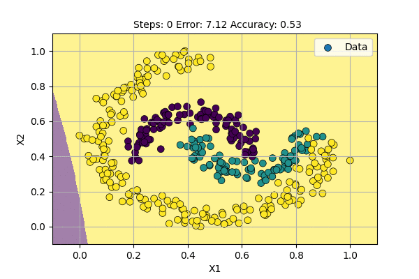
Let us use a Multilayer Perceptron (aka Neural Network) with 2 input-variables, 12 hidden-units and 3 output-variables to classify data points to 3 classes. The visualization of learning classifier is shown below.
Deep Neural Networks
If we use MLP with a single hidden layer, we can approximate any function. In practice, the number of hidden units required to approximate some complex function is huge. So huge that it is computationally expensive and not useful in practice.
The approximation property arose by addition of simple functions. As we have already discussed earlier, combining functions can create complex functions.
We can also create complex functions by composing two or more functions. Composing two function means we take output of one function as input to another. Composition of functions can be represented as follows.
Generally, composing gives us much more complex function than individual functions. We can use any differentiable functions if we want to train with gradient descent and backpropagation. The functions can be anything (MLP, Polynomial Regression, Decision Tree*, etc) as long as they are differentiable.
[Decision Trees, in general, are not differentiable. However, Soft Decision Trees are differentiable.]
Let us compose two MLPs each with 1 hidden layer. The diagram of the MLPs is as follows.

The composition of the MLPs can be shown in a diagram as follows.

Since we can combine two Linear transformations into one, our network simplifies to following.

Hence, Multilayer Perceptron with 2 hidden layers is equivalent to composing 2 MLPs each with 1 hidden layer. We can compose multiple MLPs to get multiple layers. Neural Network with many hidden layers is called as Deep Neural Network.
We can increase the number of hidden layers to increase the complexity of the function learned. We have used 2 types of operation for combining functions, superposition and composition, to create Deep Neural Network. Deep Neural Networks are trained end-to-end using Backpropagation. There were many problems while training deep networks such as vanishing and exploding gradient, slow convergence, etc. These problems were solved gradually which enabled training of very deep neural networks.
Deep Learning
Deep learning term is famous these days. It is a set of established techniques that are used to train Deep Neural Networks efficiently and easily. These techniques include the use of accelerated optimizers (RMSProp, Adam), various architectures (CNN, RNN, GAN), weight initialization (Xavier Initialization), loss functions (Cross-Entropy, MSE), Regularization (Dropout, L2) and many more.
Conclusion
In this post, we started from Perceptron, trying to improve its capability and improved until we developed the Deep Neural Network. The actual development of Deep Neural Networks did not happen exactly the same way. Still, these steps help to develop the concept in a sequential manner. Each next step adds to the capability of the algorithm. Learning this way can help try different ideas at different stages of development. Learning the modern Deep Learning algorithms can be too much for newcomers, too abstract and might be discouraging. This post aims to help readers understand the basic Neural Network algorithm and move onwards toward modern Deep Learning Techniques. Check out Linear Regression and Polynomial Regression to understand the basic of regresion.
Please feel free to comment on the post, ask questions or give feedback.